» Esercizi svolti di Matematica e Fisica

[¯|¯] L'equazione di Thomas-Fermi nel paradigma della geometria differenziale

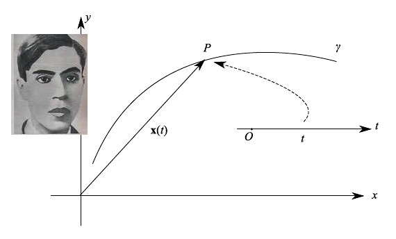
Potrebbe esserci un legame tra metodo utilizzato da Ettore Majorana per integrare la celebre equazione di Thomas-Fermi e la nozione di rappresentazione parametrica di una curva piana. Si parte passando ad una rappresentazione parametrica di una assegnata curva integrale di una equazione differenziale del secondo ordine non lineare ove non compare la derivata prima (ci stiamo riferendo a una particolare classe di equazioni differenziali a cui appartiene la Thomas-Fermi). Ovviamente non conosciamo la rappresentazione parametrica, però il punto di forza del metodo di Majorana sta nei seguenti punti: 1) una curva (regolare o meno) ammette infinite rappresentazioni parametriche; 2) solitamente si considerano in geometria differenziale, curve prive di punti multipli (ecco perché è importante il concetto di iniettività di una funzione vettoriale, e questo lo vedremo a breve anche a carattere locale).

Il punto 2 ci permette di invertire la funzione vettoriale che definisce la rappresentazione parametrica e il parametro, cioè scrivere t=t(x,y) e di queste ne ho quante ne voglio i.e. infinite, perché esistono infinite rappresentazioni parametriche di una curva assegnata. Allora si assegna tale funzione t(x,y), dopodiché si definisce una nuova funzione u=u(y,y') che poi va derivata rispetto a t. Dopo svariate manipolazioni, si giunge a un'equazione differenziale DEL PRIMO ORDINE in u(t), e questo significa che il metodo è riuscito ad abbassare di una unità l'ordine dell'equazione differenziale.

Scarica l'articolo in pdf

There could be a link between method used by Ettore Majorana to integrate the famous equation of Thomas-Fermi and the notion of parametric representation of a plane curve. We start by passing to a parametric representation of an assigned integral curve of a nonlinear second order differential equation where the first derivative does not appear (we are referring to a particular class of differential equations to which Thomas belongs - Stops). Obviously we do not know the parametric representation, but the strength of the Majorana method lies in the following points: 1) a curve (regular or not) admits infinite parametric representations; 2) usually in differential geometry, curves without multiple points are considered (this is why the concept of injectivity of a vector function is important, and we will see this shortly also of a local nature).

Point 2 allows us to invert the vector function that defines the parametric representation and the parameter, i.e. write t = t (x, y) and I have as many of these as I want i.e. infinite, because there are infinite parametric representations of an assigned curve. Then we assign this function t (x, y), after which we define a new function u = u (y, y ') which is then derived with respect to t. After several manipulations, we arrive at a FIRST ORDER differential equation in u (t), and this means that the method has succeeded in lowering the order of the differential equation by one unit.

Tags: atomo di thomas fermi, equazione di Thomas Fermi, modello di thomas fermmi